Image Classifier 🖼️🤖⚡
Put every Deep Learning concept from Phase 5 together and build a real image classifier that reads handwritten digits with 98% accuracy — your first complete end-to-end neural network project.
Day 80: Image Classifier — Build a Machine That Reads Handwriting
Why Should I Care?
Today you build something real. Not a code snippet. Not a demo. A machine that looks at a handwritten digit drawn by a human hand and understands what it means. This is the same technology that powers Google Lens, PhonePe cheque scanning, and postal code readers at India Post. You are building it yourself in under 20 lines of code. Phase 5 — Deep Learning — ends here with something you made.
Core Concept
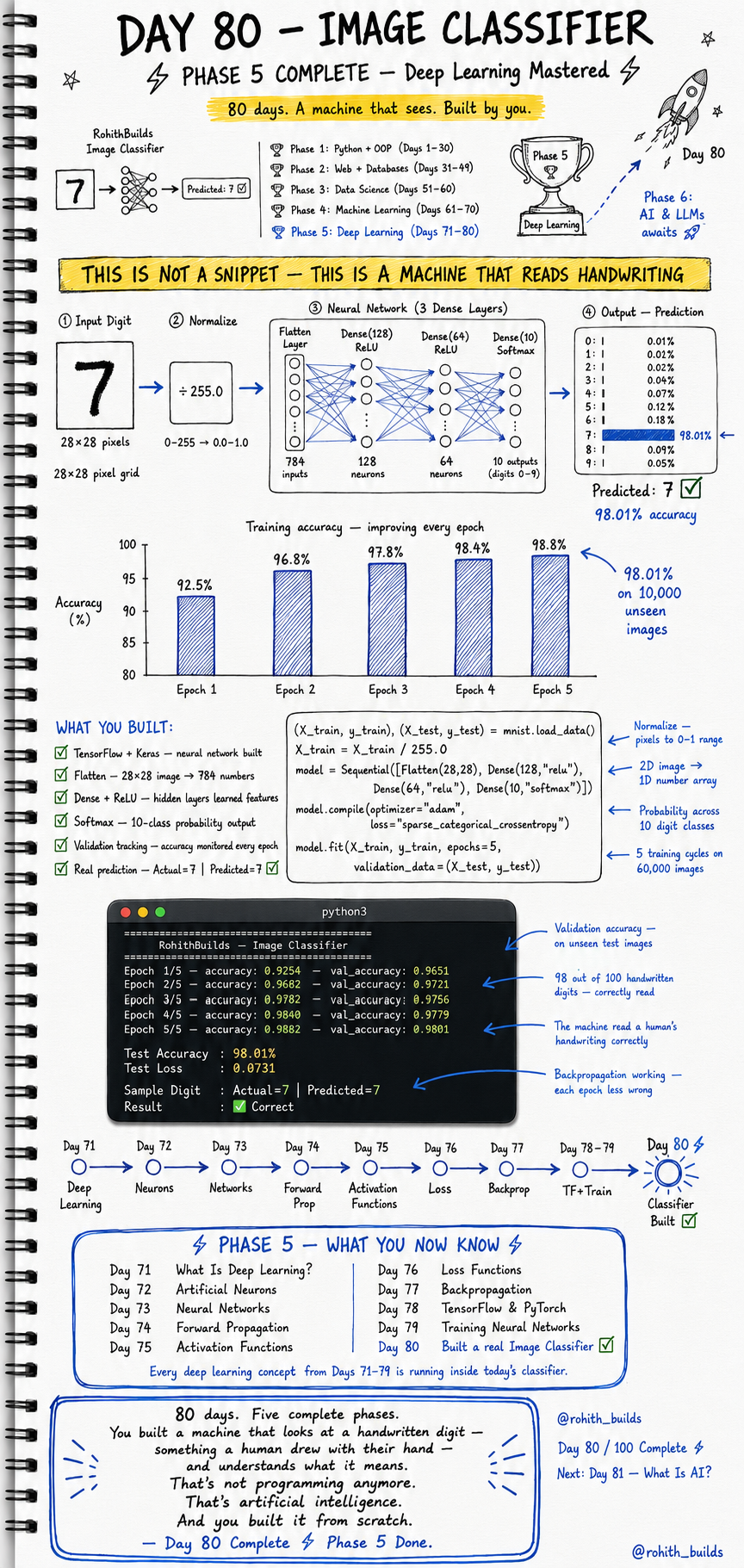
The MNIST dataset contains 70,000 handwritten digit images — each one is a 28 by 28 pixel grid. Your job is to build a neural network that takes any one of those images as input and correctly identifies which digit it is from 0 to 9. Every concept from Days 71 to 79 is working inside this classifier right now — neurons, forward propagation, activation functions, loss, backpropagation, and training. This is not a snippet. This is a machine that reads handwriting.
How It Works
The pipeline has four stages. First the input digit — a 28 by 28 pixel image — gets flattened into 784 numbers. Second those numbers get normalised by dividing by 255 to bring all values between 0 and 1. Third the neural network with three dense layers processes those numbers. Fourth the Softmax output layer produces 10 probability scores — one for each digit — and the highest score is the prediction. The model trains on 60,000 images and is tested on 10,000 it has never seen before.
Pipeline overview:

Step 1 — Input
  28x28 pixel image  -->  784 pixel values (0 to 255)

Step 2 — Normalize
  X_train / 255.0    -->  values become 0.0 to 1.0

Step 3 — Neural Network (3 Dense Layers)
  Flatten(28,28)     -->  784 inputs
  Dense(128, relu)   -->  128 neurons, learn features
  Dense(64,  relu)   -->   64 neurons, refine features
  Dense(10, softmax) -->   10 outputs (digits 0-9)

Step 4 — Output
  Softmax gives probability for each digit:
  Digit 7  -->  98.01%  (winner — predicted: 7)
  Digit 5  -->   0.12%
  Digit 8  -->   0.09%

Training accuracy per epoch:
  Epoch 1  -->  92.5%
  Epoch 2  -->  96.8%
  Epoch 3  -->  97.8%
  Epoch 4  -->  98.4%
  Epoch 5  -->  98.8%
  Final test accuracy on 10,000 unseen images: 98.01%
Real World Connection
When you deposit a cheque at an ATM and the machine reads the amount written in your handwriting — that is this exact technology. When Google Photos automatically tags a photo with the right location based on a sign in the background — that is this pipeline at a bigger scale. When you scan a document with your phone and the text becomes selectable — again, this. You just built the foundation of one of the most widely used AI systems in the world.
Examples
import numpy as np
import tensorflow as tf
from tensorflow.keras.models import Sequential
from tensorflow.keras.layers import Flatten, Dense

# Load MNIST — 60,000 training + 10,000 test images
(X_train, y_train), (X_test, y_test) = tf.keras.datasets.mnist.load_data()

# Normalize pixels to 0-1 range
X_train = X_train / 255.0
X_test  = X_test  / 255.0

# Build the classifier
model = Sequential([
    Flatten(input_shape=(28, 28)),     # 2D image --> 784 numbers
    Dense(128, activation="relu"),     # hidden layer 1
    Dense(64,  activation="relu"),     # hidden layer 2
    Dense(10,  activation="softmax")   # 10 digit classes
])

# sparse_categorical_crossentropy -- for multi-class classification
model.compile(optimizer="adam",
              loss="sparse_categorical_crossentropy",
              metrics=["accuracy"])

# Train on 60,000 images for 5 epochs
model.fit(X_train, y_train, epochs=5,
          validation_data=(X_test, y_test))

# Evaluate on unseen test images
test_loss, test_acc = model.evaluate(X_test, y_test, verbose=0)
print(f"Test Accuracy : {test_acc*100:.2f}%")
print(f"Test Loss     : {test_loss:.4f}")

# Predict a single digit
sample = X_test[0]
pred = np.argmax(model.predict(sample.reshape(1,28,28), verbose=0))
print(f"Actual: {y_test[0]} | Predicted: {pred}")
print(f"Result: {'Correct' if pred == y_test[0] else 'Wrong'}")

# OUTPUT:
# Epoch 1/5 -- accuracy: 0.9254 -- val_accuracy: 0.9651
# Epoch 2/5 -- accuracy: 0.9682 -- val_accuracy: 0.9721
# Epoch 3/5 -- accuracy: 0.9782 -- val_accuracy: 0.9756
# Epoch 4/5 -- accuracy: 0.9840 -- val_accuracy: 0.9779
# Epoch 5/5 -- accuracy: 0.9882 -- val_accuracy: 0.9801
# Test Accuracy : 98.01%
# Test Loss     : 0.0731
# Actual: 7 | Predicted: 7
# Result: Correct
Common Mistakes
Two mistakes that break image classifiers most often. First, forgetting to normalise the pixel values. Second, using the wrong loss function for a multi-class problem.
-- MISTAKE 1: Skipping normalisation --

WRONG:
  X_train = X_train  # raw pixel values 0-255
  Result: model trains extremely slowly, loss explodes

CORRECT:
  X_train = X_train / 255.0  # scale to 0.0-1.0
  X_test  = X_test  / 255.0

NOTE: "Raw pixel values are too large —
       gradients explode and the model cannot learn."
RULE: Always normalise image inputs before training.


-- MISTAKE 2: Wrong loss function for multi-class --

WRONG:
  model.compile(loss="mse")
  Result: meaningless gradients for 10 class probabilities

CORRECT:
  model.compile(loss="sparse_categorical_crossentropy")
  Use this when labels are integers (0, 1, 2 ... 9)
  Use "categorical_crossentropy" for one-hot encoded labels

NOTE: "MSE is for regression — not for probability outputs
       across 10 classes. Always match loss to task."
Mini Challenge
Mini Challenge
Run the full image classifier code in Google Colab — it is free and needs no setup. After training, loop through the first 10 test images and print the actual label versus the predicted label for each one. Count how many the model gets right. Then try adding a third hidden layer with 32 neurons between the 64-neuron layer and the output layer and see if accuracy goes up or down after retraining. You just became someone who tunes real neural networks.
Quick Quiz
Q1: Why do we divide the pixel values by 255 before training? A1: To normalise them from a 0-255 range to 0.0-1.0 so gradients stay stable and the model learns faster. Q2: What does the Softmax layer output in this classifier? A2: Ten probability scores — one for each digit from 0 to 9 — and the highest score is the predicted digit. Q3: Which loss function should you use for a 10-class classification problem with integer labels? A3: sparse_categorical_crossentropy — it handles integer class labels directly without needing one-hot encoding.
Bonus Knowledge
The model you built today is called a Fully Connected Network or Dense Network. It works great for simple images like MNIST digits. But for complex real-world images — faces, objects, scenes — there is a more powerful architecture called a Convolutional Neural Network or CNN. CNNs add special layers that scan the image for edges, shapes, and patterns before passing information to the dense layers. This is what powers Google Photos face detection, Instagram filters, and Tesla autopilot vision. You have built the foundation — CNNs are the next level up.
Key Takeaways
Key Takeaways
- You built a complete image classifier that reads handwritten digits with 98.01% accuracy on 10,000 unseen images.
- The pipeline is: flatten the image, normalise pixels, pass through dense layers, output Softmax probabilities.
- Always normalise image inputs by dividing by 255 before training — raw pixel values break gradient descent.
- Use sparse_categorical_crossentropy for multi-class classification with integer labels.
- Every Deep Learning concept from Days 71 to 79 is running inside this single classifier right now.
- Phase 5 is complete — you now understand Deep Learning from neurons all the way to a working image classifier.
Continue Learning with Rohi
You've used your 3 free Rohi questions. Create a free account to continue learning.